
In a previous article we presented the concept of hypothesis testing—a statistical method widely used to determine the validity of a claim based on a sample of data.
In the examples we proposed, however, we knew the value of the population standard deviation, sigma. In practice, this is a rather rare case, which allowed us to use the normal distribution and compute the Z-score.
If instead we do not know the population sigma, or if we are working with small samples, we must turn to a different type of distribution, called the t distribution or Student’s distribution.
Put more simply and clearly:
Student’s t distribution is a probability distribution used to assess the statistical significance of results when dealing with small sample sizes and uncertainty about the variance.
What We’ll Cover
A Brief Historical Digression
In the early 1900s, the chemist and statistician William Sealy Gosset, employed at the Guinness brewery (and a collaborator of the statistical giant Karl Pearson), discovered that when working with very small samples, the distributions of the mean differed significantly from the normal distribution.
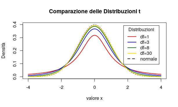
Even more interesting, as the sample size changed, the shape of the distribution changed too, and as the sample grew, the distribution gradually approximated the normal more and more closely.
Unable to reveal his identity so as not to benefit competitors, he published his results under the pseudonym “Student”—and this is why distributions for small samples are now known as “Student’s t distributions.” If you want to read the full story, Wikipedia is, as always, a good source.
The t distribution is symmetric about zero, but it is “flatter” than the standardised normal distribution, so that a greater portion of its area lies in the tails.
A larger sample causes the t distribution to approximate the normal distribution ever more closely. The differences between the t distribution and the normal are greatest when we have fewer degrees of freedom.
But what do we mean by degrees of freedom? The number of sample values that have the “freedom” to change without altering the sample mean.
If the concept is not immediately clear, we can still move on to practical usage, because the degrees of freedom—fundamental to our calculation—are simply equal to the sample size minus one:
df = n – 1
where df = degrees of freedom
n = sample size
The procedure for conducting a hypothesis test using the t distribution largely mirrors what we have already seen in the case of a known sigma and the use of the normal distribution.
We therefore state the null hypothesis, H0, and the alternative hypothesis, Ha.
To compute the t-test statistic we use the formula:
\(t = \frac{\bar{x} – \mu}{\frac{s}{\sqrt{n}}} \\
\)
where \(\frac{s}{\sqrt{n}}\) is the estimated standard error, which we can also denote as SE.
An Example Is Worth a Thousand Explanations
A light bulb manufacturer claims that its product has a mean lifespan of at least 4200 hours.
A sample of n = 10 bulbs is taken, and the sample mean lifespan is found to be 4000 hours. The sample standard deviation is 200 hours.
In summary:
\(n=10 \\
\bar{x}=4000 \\
s=200 \\
\)
We then set up our test conditions:
H0: μ ≥ 4200
Ha: μ < 4200
We choose a significance level of 95% (i.e. alpha = 0.05).
In the table of critical values for the t distribution, we look up the value corresponding to 9 degrees of freedom (the row) and alpha 0.05 (cross with the column). This value turns out to be 1.833.
We will reject the null hypothesis if the t value we calculate is less than -1.833.
The standard error is:
\(\frac{s}{\sqrt{n}}=\frac{200}{\sqrt{10}}=\frac{200}{3.16}=63.3 \\
\)
We compute t:
\(t=\frac{\bar{x} – \mu}{SE}=\frac{4000-4200}{63.3}=\frac{-200}{63.3}=-3.16 \\
\)
The t value falls in the critical region: we therefore reject the null hypothesis and accept, at a 95% significance level, that the mean bulb lifespan is less than the 4200 hours claimed by the manufacturer.
An Alternative to Critical Regions: Looking at the p-Value
We can also evaluate a hypothesis by asking: “What is the probability of obtaining the test statistic value we observed, if the null hypothesis is true?” This probability is called the p-value.
This is, in fact, the most convenient approach when we have tools such as a statistical calculator or R: the interpretation of the result is immediate.
Using R or a calculator on our example, we obtain t = -3.16 and p = 0.00575.
This means there is just a 0.575% probability that under the null hypothesis we would observe the result we found.
p is less than our chosen significance level alpha (p < 0.05).
Therefore, the null hypothesis is to be rejected in favour of the alternative hypothesis.
Estimate, Margin of Error, and Confidence Interval: Verifying the Hypothesis Test Result
When a hypothesis is rejected, it is certainly useful to produce an estimate to try to understand what the true mean value is. In our example, we rejected the manufacturer’s claim that their bulbs last on average more than 4200 hours. But then, how long do they actually last?
To calculate the confidence interval, we need to know three things:
- The sample mean
- The standard error
- The critical value
The formula for the confidence interval is:
\(\bar{x} \pm Margin\ of\ Error \\
\)
and the Margin of Error is:
\(ME = t_{critical} \times SE \\
\)
In our case: ME = 1.833 × 63.3 ≈ 116
So we can say that our 95% confidence interval is between 3884 and 4116.
As we can see, the value stated by the manufacturer, 4200 hours, falls—as we expected—outside the confidence interval.
The t-Test, p-Value, and Confidence Interval in R
R is, as always, our best ally, allowing us to perform the test with utmost simplicity and providing all the information we need. We prepare a vector containing 10 measurements with a mean of 4000 and feed it to R’s t.test function, specifying that the null hypothesis mean (mu) is 4200, and that the alternative hypothesis is that the true value is lower—alternative = “less”:
bulb_life <- c(4100, 3900, 3800, 4200, 4000,
               4100, 3900, 3800, 4200, 4000)
t.test(bulb_life, mu = 4200, alternative = "less")
R provides in its output all the information we need: the t statistic, the p-value, and the confidence interval.
In general, Student's t distribution is a powerful and flexible tool that can be used to assess the statistical significance of results in many different contexts. With a thorough understanding of the t distribution and the use of software like R, it is possible to construct effective hypothesis tests and make informed decisions based on the data collected.
Side note: if the sample is small (n < 30) and the population is not approximately normally distributed, we can apply Chebyshev's Theorem.
Useful Links for Further Study
- How t-Tests Work: t-Values, t-Distributions, and Probabilities — statisticsbyjim.com
- One Sample T Hypothesis Test (Student's T Test) — sixsigmastudyguide.com
You might also like
- Hypothesis Testing: A Step-by-Step Guide
- Confidence Intervals: What They Are, How to Calculate Them (and What They Do NOT Mean)
- Guide to Statistical Tests for A/B Analysis
Further Reading
For a comprehensive treatment of the t distribution, hypothesis testing, and the full machinery of statistical inference, Statistica by Newbold, Carlson and Thorne provides a rigorous yet accessible walkthrough of the theory and practice, from small-sample tests to confidence interval construction.