Descriptive Statistics: Measures of Variability (or Dispersion)

Measures of variability are used to describe the degree of dispersion of observations around a central tendency index.

In other words, measures of variability allow us to assess how data are spread around a central value, which may be represented, for example, by the mean or the median. They provide valuable information about the distribution of data, enabling a better understanding of the phenomenon under observation.

The techniques for measuring the variability of datasets are numerous. Among them, the most widely known (and most commonly used) are:

the range
the mean deviation and the variance
the standard deviation
the coefficient of variation

We will also visualise the concepts of central tendency and dispersion by revisiting skewness and introducing the concept of kurtosis.

The Range

The range is the difference between the maximum and the minimum value of ungrouped data in a frequency distribution.

It is a very quick calculation, which in R can be computed as follows:

max(var) - min(var)

The maximum and minimum can also be displayed with:

range(var)

and they appear as the first and last terms in:

fivenum(var)

For grouped data, the range is defined as the difference between the upper boundary of the highest class and the lower boundary of the lowest class.

A trimmed range is a range from which a certain percentage of extreme values has been removed from both ends of the distribution (for instance, the middle 80 per cent).

The Mean Deviation

The mean deviation is a measure of variability based on the difference between each data point and the mean. If we calculated the average by summing the positive and negative differences between each value and the arithmetic mean, the result would always be zero. For this reason, we sum the absolute values of the differences:

\(
SM = \frac{\Sigma|X – \mu|}{N} \\
\)

Those “absolute values” pose some computational efficiency issues, which is why the mean deviation is not widely used. There is another way to eliminate negative values, and so we introduce the important concept of…

Variance

Variance is analogous to the mean deviation, since it is based on the differences between each data point and the mean, but these differences are squared before being summed. Variance is denoted by the lowercase sigma squared symbol, and the formula is:

\(
\sigma^{2}=\frac{\Sigma(X – \mu)^{2}}{N} \\ \\
\)

R has the var() function for computing variance, but it uses (n-1) in the denominator. To obtain the variance with N in the denominator, we can define a custom function:

pop_var <- function(x) { var(x) * (1 - 1/length(x)) }

In general, interpreting the value of a variance is difficult because the units it is expressed in are not the same as those of the original observations.

For this reason, the standard deviation was introduced.

The Standard Deviation: The Most Widely Used Measure of Variability

The standard deviation is simply the square root of the variance:

\(
\sigma = \sqrt{\frac{\Sigma(X - \mu)^{2}}{N}} \\ \\
\)

The standard deviation is of fundamental utility in statistics, particularly (as we shall see) in conjunction with the normal distribution.

For grouped data, we assume that the midpoint of each class represents all the measurements within that class. The variance formula then becomes:

\(
\sigma^{2}=\frac{\Sigma f(X - \mu)^{2}}{N} \\ \\
\)

and the standard deviation:

\(
\sigma = \sqrt{\frac{\Sigma f(X - \mu)^{2}}{N}} \\ \\
\)

In R, the function for computing the standard deviation is sd(). However, R uses (n-1) in the denominator. So, if we want the population standard deviation (with n in the denominator), we can define a dedicated function:

pop_sd <- function(x) { sqrt(sum((x - mean(x))^2) / length(x)) }

The Coefficient of Variation

The coefficient of variation indicates the relative magnitude of the standard deviation with respect to the distribution mean. It is extremely useful for comparing phenomena expressed in different units of measurement, since the CV is a "pure" number, independent of the unit of measurement:

\(
CV = \frac{\sigma}{\mu} \\
\)

As is often the case in R, there is a ready-made function: we can use cv(), defined in an external library, labstatR. Its usage is straightforward:

library(labstatR)
data <- c(24, 17, 21, 23, 15, 30, 24, 21, 24, 19,
          25, 28, 22, 20, 14, 19, 26, 29, 23, 25,
          24, 18, 27, 21)
cv(data)
# [1] 0.1817708

We can also calculate the value quite simply without resorting to external libraries:

data <- c(24, 17, 21, 23, 15, 30, 24, 21, 24, 19,
          25, 28, 22, 20, 14, 19, 26, 29, 23, 25,
          24, 18, 27, 21)
pop_sd <- function(x) { sqrt(sum((x - mean(x))^2) / length(x)) }
cv_data <- pop_sd(data) / mean(data)
cv_data
# [1] 0.1817708

The Shape of a Distribution

Frequency distributions can take on the most varied shapes. Among all of them, the one by far most important in statistics is the normal distribution, also known as the bell curve or Gaussian distribution.

In a normal distribution, data are arranged symmetrically around the mean. In a very straightforward way, to describe the shape of the distribution we simply compare the mean with the median: if they are equal, the distribution is symmetric. If the mean is greater than the median, we have positive skewness (with a longer "tail" on the right); if the mean is less than the median, the skewness is negative (with the longer "tail" on the left).

The best-known formula for calculating the skewness of a distribution is Pearson's coefficient of skewness:

\(
Skewness = \frac{3(\mu - med)}{\sigma} \\ \\
\)

A perfectly symmetric distribution has a skewness value of 0. A right-skewed (positive) distribution has a positive value, while a left-skewed distribution has a negative value.

Skewness values typically fall between -3 and 3, and the fact that the standard deviation appears in the denominator makes the value independent of the unit of measurement.

How do we calculate the skewness index in R? The simplest way is to use a library that provides the functions we need "ready to go":

library(moments)
data <- c(24, 17, 21, 23, 15, 30, 24, 21, 24, 19,
          25, 28, 22, 20, 14, 19, 26, 29, 23, 25,
          24, 18, 27, 21)
skewness(data)
# [1] -0.1918578

The moments library serves us well. Let us see, however, how to calculate the index without relying on a library. It is very simple. The first step is to remember that R uses n-1 in the denominator of the variance. We are reasoning about a population, however, with n in the denominator. So, let us define a function that gives us the value we need:

pop_var <- function(x) { var(x) * (1 - 1/length(x)) }

At this point we can calculate the skewness index:

data <- c(24, 17, 21, 23, 15, 30, 24, 21, 24, 19,
          25, 28, 22, 20, 14, 19, 26, 29, 23, 25,
          24, 18, 27, 21)
pop_var <- function(x) { var(x) * (1 - 1/length(x)) }
z <- (data - mean(data)) / sqrt(pop_var(data))
skew <- mean(z^3)
skew
# [1] -0.1918578

Kurtosis

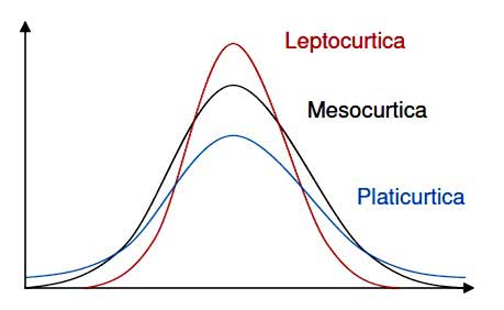
Kurtosis is the degree of peakedness of a distribution curve, relative to the normal distribution.

We have three cases:

a tall curve, called leptokurtic, which is highly concentrated around its mean
a normal curve, called mesokurtic
a low and flat curve, called platykurtic, with little concentration around its mean

Measures of variability: leptokurtic, mesokurtic, and platykurtic curves

Kurtosis can be measured by dividing the fourth moment by the standard deviation raised to the fourth power. Sounds difficult? It is easier done than said. Here is the formula:

\(
Kurtosis = \frac{\Sigma f(X -\mu)^{4}}{\sigma^{4}} \\ \\
\)

The kurtosis of a mesokurtic curve has a value of 3. Naturally, a kurtosis coefficient less than 3 indicates a platykurtic curve, while a value greater than 3 indicates a leptokurtic curve.

As with the skewness index, the moments library provides a convenient ready-made function:

library(moments)
data <- c(24, 17, 21, 23, 15, 30, 24, 21, 24, 19,
          25, 28, 22, 20, 14, 19, 26, 29, 23, 25,
          24, 18, 27, 21)
kurtosis(data)
# [1] 2.480035

But we are not averse to computing it ourselves:

data <- c(24, 17, 21, 23, 15, 30, 24, 21, 24, 19,
          25, 28, 22, 20, 14, 19, 26, 29, 23, 25,
          24, 18, 27, 21)
pop_var <- function(x) { var(x) * (1 - 1/length(x)) }
z <- (data - mean(data)) / sqrt(pop_var(data))
kurt <- mean(z^4)
kurt
# [1] 2.480035

We have seen that measures of central tendency alone are not enough: two datasets can have the same mean yet behave in profoundly different ways. Variability tells us how much the data fluctuate, and the shape of the distribution tells us how they are arranged. In the next article, we will take the first steps into the world of probability—the essential bridge between descriptive statistics and the inferential tools that let us draw conclusions from data.